Smooth particle mesh Ewald (SPME) is a method of calculating long range interactions like gravity and electrostatics for molecular dynamics (MD) simulations. This calculation is essential to get accurate simulations, but is often the most expensive component and is a natural candidate for parallelization. To accelerate the SPME calculation we implement the energy and force calculation on a GPU using CUDA.jl. This requires three kernels: the real space sum, charge interpolation and the reciprocal space sum. In the real space sum we demonstrate linear scaling and a 4x speed-up compared to a commercial MD code by building a spatially sorted neighbor list. Combining all three kernels, we achieve a 6x speed-up for the largest system tested. For even larger systems our code will continue to outperform the CPU implemented and achieve better speed-ups greater than the number of CPU cores.
Work Distribution: Ethan completed the real space sum and benchmarks, Nick completed the reciprocal space sum and charge interpolation. All other work (writing etc.) was split evenly.
The theory and equations of Smooth Particle Mesh Ewald can be found in our full report inside of the GitHub repository (here) as well as in the original paper which can be found here
To implement SPME on a GPU, we used the CUDA.jl wrapper of the CUDA C-API. This warpper provides the conveniences of a high level language (Julia) while retaining all the kernel programming functionality of CUDA. CUDA.jl helped us avoid common issues like segmentation faults, as there are no raw pointers in Julia, and accelerated the development process by removing code compilation.
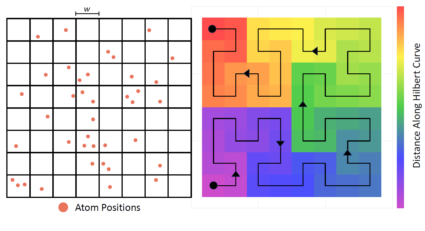
The implementation of the real space sum follows the OpenMM kernel for non-bonded interactions. This kernel is generic and capable of calculating the interaction of any potential, not just electrostatics. Before execution, this kernel requires a custom neighbor list that maps well onto GPU hardware. The steps to build this neighbor list are:
The final step to build the neighbor list is $\mathcal{O}(N^2)$; however, the neighbor list only needs to be re-built every 100 time steps. The computational complexity of the real space sum will be dominated by the GPU kernel. Note that the neighbor list is built on CPU, but these kernels could be ported to GPU as well.
The CUDA kernel is launched with one thread block for every pair of interacting bounding boxes each with 32 threads. Within each block the positions of the 32 atoms in each bounding box are moved into shared memory (384 bytes). Then one of three kernels is selected to calculate the force and energy. If the pair of bounding boxes contains the same two bounding boxes, then only half of the interactions need to be calculated to avoid double counting (528 interactions). The next scenario checks the flag calculated in step 6. If more than 24 atoms are flagged as non-interacting, the kernel only calculates the non-flagged interactions. This requires a reduction across the warp at each step as it cannot be guaranteed that the warp will not diverge. Otherwise, all 1024 interactions are calculated. Inside of each warp the interactions are calculated in a staggered fashion, so that there is no warp divergence and each thread calculates interactions independent of other threads.
The figure below shows the scaling of our GPU real space kernel with the number of atoms compared to LAMMPS on 1 CPU-core. Both codes exhibit linear scaling, but the GPU code has a lower constant factor and becomes a better option than the CPU around 1000 atoms.
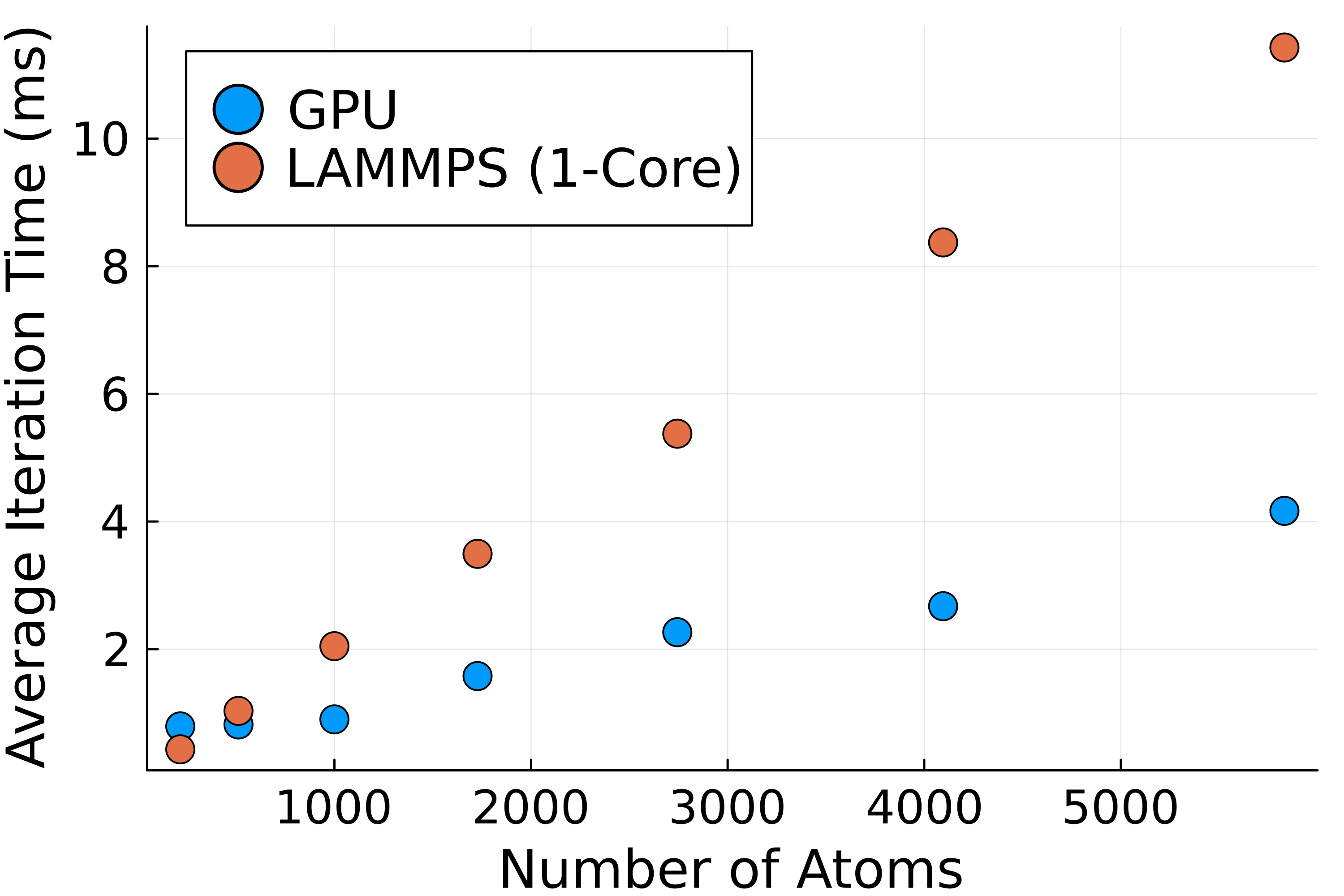
For the last data point, which represents a 9x9x9 unit cell salt crystal with 5832 atoms, we also ran several MPI simulations of LAMMPS to determine how many cores it took to match a single GPU. Due to the highly optimized nature of LAMMPS, the CPU code scaled almost perfectly with the number of atoms and only required 4 cores to match the GPU. This may not sound like a big win for the GPU; however, molecular dynamics code does not map well to the GPU and single-digit speed-ups are expected. Furthermore, due to the different constant factors, the speed-up gained by using a GPU will only cont
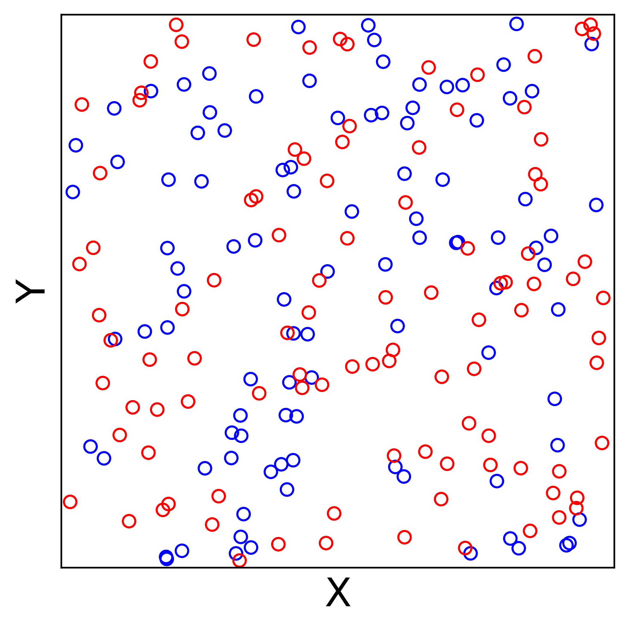
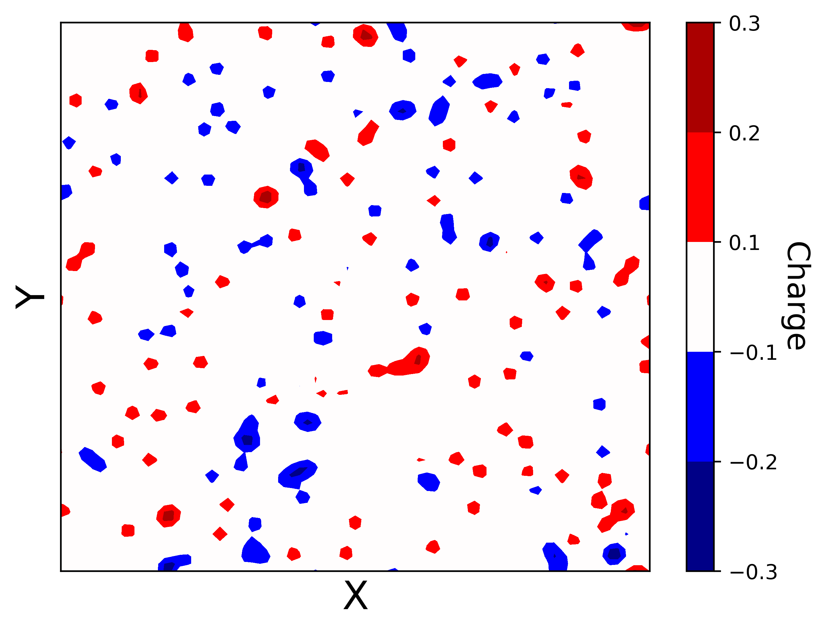
Before the reciprocal space sum can be performed, the discrete set of point charges must be interpolated onto a regular grid of mesh points. This allows us to use a Fast Fourier Transform (FFT) to approximate the structure factor \(S(\vec{m})\) in and accumulate the reciprocal space energies in \(\mathcal{O}(N\log(N))\). The figure below shows the process of spreading out a set of randomly chosen point charges. The use of nth order B-splines guarantees the interpolated charge field is \(n-2\) times differentiable, which means forces can be analytically derived from the energy expressions in Eqns.
An example of interpolating a set of discrete charges onto a regular mesh grid. This has the effect of "spreading" the point charges out.
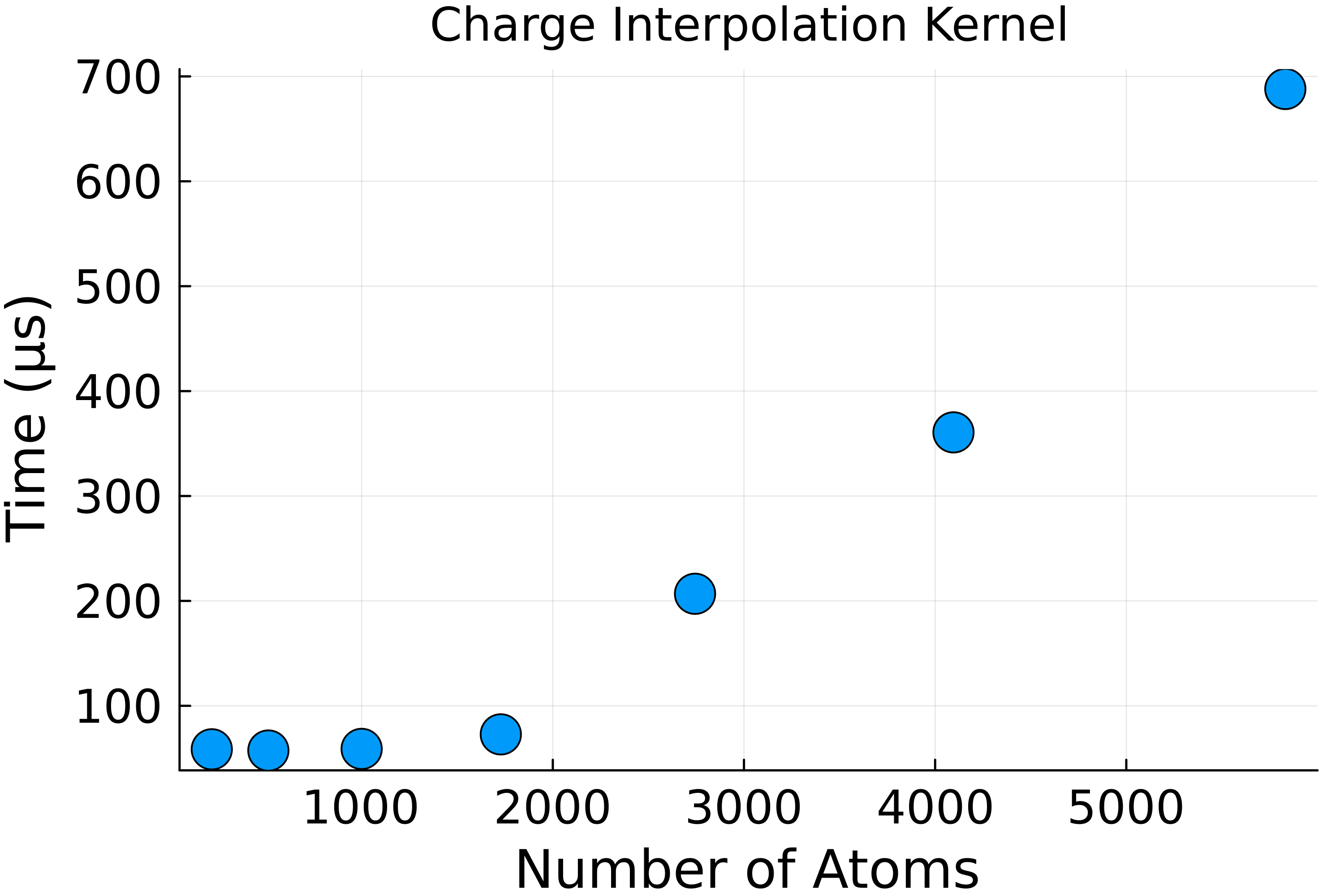
To interpolate the charge on GPU, we assigned one thread to every atom in the system with a block size of 64. The small block size was chosen as the number of atoms in the system was on the order of 1000, and it is better to launch multiple blocks to fully saturate the GPU's compute capabilities. Each thread calculated an atom's contribution to the \(n^3\) neighboring mesh points. Because multiple atoms can contribute to the same cell, we used the atomic add operation to avoid data races.
The charge interpolation kernel was tested with the same salt crystals and showed the expected linear scaling with the number of atoms as shown in Fig 1. The first few data points do not scale well as the kernel launch time is comparable to the compute time, and only a few streaming multiprocessors (SMs) are active.
The reciprocal space took advantage of the high-level Julia wrapper of the FFTW library to call the CuFFT library. We simply moved the interpolated charge array to the GPU and called the appropriate FFT and IFFT functions. To optimize the calculation, we chose the mesh spacing to be a factor of 2, 3, or 5 as stated by the CUDA documentation.
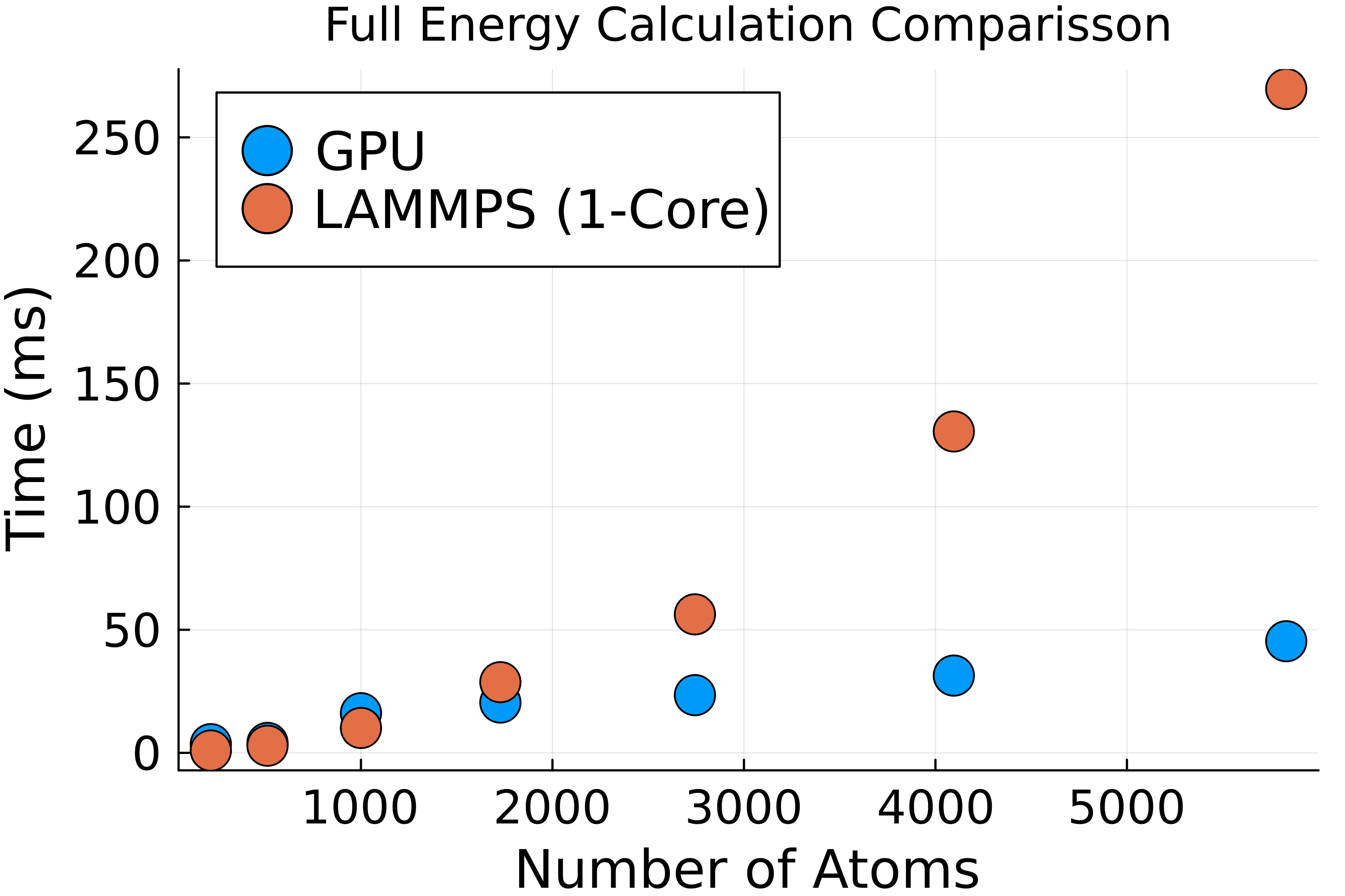
Combining the real space, charge interpolation, and reciprocal space into one code, we observe a final scaling that matches LAMMPS with a lower constant factor. Figure 5 shows the comparison of the energy loop in LAMMPS compared to our energy loop on a GPU. Both show \(N\log N\) scaling, demonstrating the importance of the FFT code. Our GPU code outperforms the LAMMPS simulation with a speed-up of 6x at 9 unit cells. The performance gap will continue to grow as the system size increases, demonstrating the importance of using a GPU to run large MD simulations. For the systems studied here, adding extra CPU cores will allow the CPU code to easily match the GPU code; however, in systems with many tens of thousands of atoms, the GPU speed-up will be more than the number of cores on a CPU.
We successfully implemented SPME on a GPU using the CUDA.jl library. Our code not only demonstrates the superiority of GPU’s for large-scale MD simula- tions, but also the maturity of the Julia ecosystem for GPU programming. In the salt system tested, the GPU routinely outperformed the LAMMPS program when the system had more than 1000 atoms with a maximum speed up of 6x for the 9 unit cell system. The main bottleneck in our code is the FFT implementation which has NlogN scaling. This kernel cannot be optimized much as it is part of the CUDA library; however, we can hide that computational cost by performing computation on the CPU at the same time or by using multiple GPUs. In the future, we would like to add support for multiple GPU’s and also make it agnostic of which GPU back-end is used (e.g. CUDA vs. AMD). Furthermore, optimizing the real-space kernel would have benefits beyond SPME. This kernel is generally useful for all non-bonded MD interactions and could ac- celerate other portions of the simulation. With these changes our code could rival the speed and flexibility of other GPU codes like OpenMM and GROMACS.